Sunday, October 29, 2023

Setting Up a Student Sheet for Success

 Setting up a sheet well for someone else to use, whether that sheet is for students or teachers, can make or break its success. This post will focus on conventions that I use to make my sheets easier for users. That being said, just as curb cutouts started as a way to make sidewalks easier for differently abled people, they actually help everyone. These conventions will help everyone who uses the sheet, including you!


Often organization elements are left with header color and alternating rows. This isn’t surprising because traditional spreadsheets are table based - basically accounting tools. This is leaving a lot of the table, especially if you are working with folks who have limited spreadsheet experience. Take the two examples below of the same gradebook template. This template is meant to be used by middle school students. 
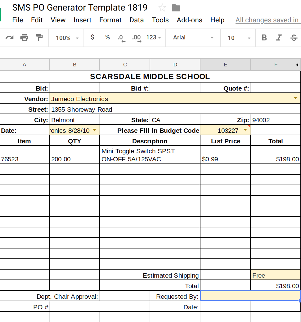
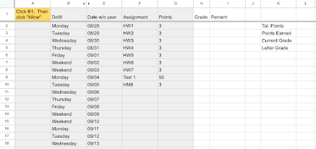

Example 1


Example 2


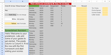
Here the goal is to teach students some introductory spreadsheet calculation skills. I would argue that the first example is opaque and even anxiety provoking. The second example uses color to focus attention on important elements, includes a Key to give the user context, and even uses a “Spreadsheet Assistant.” This handy box contains an IF/THEN/ELSE statement that changes as the user begins to build the sheet, giving the student a sequence of steps. Doing it this way takes more set up time, but it will save you and your students so much frustration on the other side. This tutorial will briefly talk about using color, making an IF/THEN assistant, locking elements so that users don’t change the wrong thing, creating a data feed, and will introduce a discussion about distribution.

Lets Talk Color and Merging

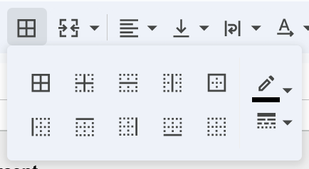
We are visual creatures. I love a good table but only when I need to organize lots of data. All those columns and rows can be visual noise if your project is more of an interface. Simply put, making the cell and border colors the same creates a cleaner visual experience. The lines can disappear where they aren’t needed. Cells can be merged to create specific areas with a larger text box, as with the spreadsheet assistant in the example. The border tool can add an underline, bring all the rows back, or simply create a box around an area, like in the Sheet Key example above.


The IF/THEN Assistant

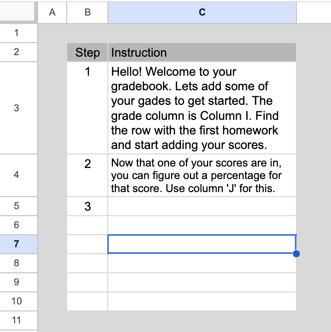
IF/THEN statements are incredibly powerful and can be very complex. These statements can look for matches, include OR statements, employ mathematical formulas, and so much more. The statement that creates the Spreadsheet Assistant can be quite simple. First, consider the steps that you would like your students to follow. Make a chart on your variables tab with a step number column and an instruction column and start to brainstorm a lesson sequence. You can type these directions directly into the IF/THEN statement but I find using a chart easier to plan and edit later.


Once your instructions are laid out, the statement is easy to compose. The syntax of an IF/THEN/ELSE statement is:

IF(logical_expression, value_if_true, else)

My first instruction looks to see if any scores have been added to the score column (I). I’ll do this by using a SUM function for the entire range, just in case a student adds a score next to a date further down the list. If the sum is less than 1, then the assistant box will contain instructions for step one on the variables sheet (Variables!C3):

=IF( SUM(I3:I)<1,Variables!C3,

My ELSE statement will be the condition for the next instruction. In this case, whether or not any percentages have been added to column J. If not, the second instruction will load (Variables!C4):


=IF( SUM(I3:I)<1,Variables!C3, IF( SUM(J3:J)<1, Variables!C4,))

And so on! The nested IF/THEN statement can provide steps for the entire project!

Locking Elements

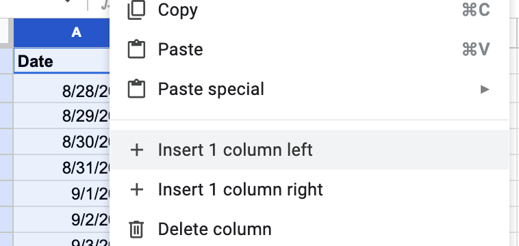
We will use a tool called Autocrat to distribute copies of the gradebook template to each student in your classes. When we do this, you will retain ownership of each sheet and you can control the level of sharing that you students possess. In this case, each student will be an editor. Because of this, you can lock particular sheets, ranges, even specific cells, that the students won’t be able to edit. Some careful consideration should be made into what cells are locked. With our gradebook, we can lock everything in the columns between A and H. Those will be teacher columns. We also want to protect the Variables sheet, at a minimum. When the sheet is distributed to your class, these protections will be maintained. Google provides a nice guide to protecting sheets and ranges here.


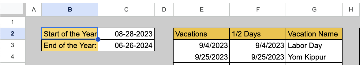
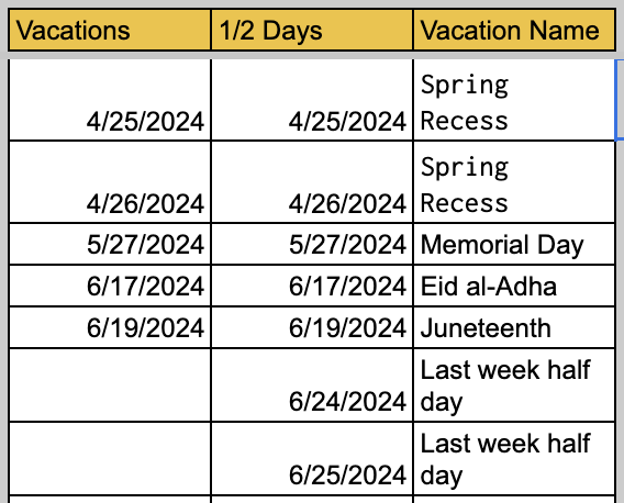
Creating a Data Feed

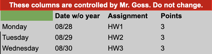
The gradebook has to be useful and easy to use. One way to do this is by feeding in data and reducing the amount of text input for students. We are going to feed in the dates for the school year, the days of the week for those dates, the assignments and tests corresponding to the dates, and the maximum score possible for each. All of this information is fed from a master sheet. The master sheet is a lesson unto itself.  This automatically creates a list of dates between two given variables, making it easy to reuse each year. You can read about how to build it here. The data is instantly sent to each student’s sheet whenever the teacher adds an assignment to the master and setting it up is easy. We will be using a function name IMPORTRANGE which allows you to pull data from a different sheet. The source sheet must be shared with the user in order for the import to work. None of this data is sensitive so it will be easy to share the source sheet as read only. We can turn off notifications, too, so that it doesn’t send an email when shared. The syntax for import range is simple:


=IMPORTRANGE(spreadsheet_url, range_string)


The first condition is the url of the source sheet, surrounded by quotes. The second condition is the location of the data range in the sheet, also surrounded by quotes:


=IMPORTRANGE("https://docs.google.com/spreadsheets/d/1UBVC6dwwH1UGnR91do-bu4RV8xM9CsTh_2oJPw-Vhdg/edit#gid=1017551313", "Scheduler!C3:H294")


There will be no data when the student opens the gradebook for the first time. The student must give permission to the connection. I usually create cues to help this process. In our example sheet I write “Click B1 & then “Allow Access” and point to cell B1 which I have made green. When a student does this (even though it is protected and the student can’t change the function) a button will appear requesting him or her to “Allow Access.” The data will feed in once access is granted!


Distribution

You cannot distribute your sheet to your class until it is completely ready. We will have a separate tutorial later about using the Autocrat extension for this purpose. In the meantime, you can set up a spreadsheet with your class rosters. This sheet will need a row for each student. The data should include the student’s first and last name, and email address at a minimum. Additional useful information could include period number, parent email (you could share it with parent as a read only doc,) learning resource teacher or case manager email, and more. When autocrat is run you will have a handy link to each student’s gradebook added to each row.


Next time we will work with an autocrat and go into the details regarding document distribution.


Extension activity:

Create a sheet in the gradebook with useful information for your students. Add a chart with the grading scale, create a reference for math symbols and share where to find them on the keyboard(^ is Shift + "6"), provide a list of tips for writing a math function (eg: All formulas must start with an equal sign)

Saturday, October 28, 2023

Building a Curriculum System - Part1: The Calendar

I often need to match a Sheets system to our school calendar. This tutorial will explain how to create a a list of dates between two variables (the start and end of a school year) and indicate which days are holidays, conference days, and half days. Just as importantly, the variables make it easy to reuse each year. This system is the core of some of my more complex projects. It is the centerpiece of my Google sheet curriculum project as well as the  scheduling platform that I use to organize student hosts for our Middle School News broadcast.


First, let's set up the pages that we will need in our spreadsheet. With the exception of a Variables page, you usually don’t want to put more than one data table on a page. Below is a bulleted list of the pages you should create and the purposes those pages will fill.

Lessons

This is an optional page. The “Lessons” page will allow you to select lessons from a drop down to change your lesson sequence. It would also allow you to link other things to the lesson, like a description, SWBATD information, and resources folders.


Instructional Days

This page will list each instructional day and assign a sequential number to each day in the list. This will allow you to shift lessons or assignments if your plan changes.


Variables

Create a variables page. This will store the start and end date for the school year. It will also contain the dates for holidays and conference days.


Setting up the calendar


Setting your Variables.

We are going to set the system up to list all the days in the school year in a vertical column. We are also going to create a flag when there is a holiday, superintendent conference day, or half day. We are going to set these values on the “Variables” pages because they will change from year to year. Let's get started.


Click on the “Variables” page. Select a cell and label it “Start of the Year.” Record the start date (Month-day-year) in the right adjacent cell. Go down a row and do the same thing for the “End of the Year.”


IMPORTANT NOTE: I am using cells C3 and C3 for my start and end dates. These cells will be represented in the function below.You will have to adjust the function in the next step if you use different cells.


Skip a column on the right and record the following three headings: 

Vacations | ½ days | Vacation Name


Fill out the “Vacations” chart. Every vacation day needs an entry. If Spring break is a week long it will require five represented days. Half days only get a date in the “Half day column.” Regular days off will have a date in both the “Vacations” column and the “½ day” column.

Building Your List of Dates


Now navigate to your “Instructional Days” sheet.  Add a heading in cell A1 named “Dates.” I am going to add an advanced function in cell A2 that will use the start and end dates on the “variables” page to build a list of dates. The beauty of this is I can change those variables next year and the list will update! I will paste the function below and then explain what it does. Full disclosure: I will use the ChatGPT AI to break down the function and then I will edit the AI response (I did need quite a bit of editing), because it is a time saver.


Function in A1: =ArrayFormula(TO_DATE(row(indirect("C"&Variables!C2):indirect("C"&Variables!C3))))


1. indirect("C"&Variables!C2):indirect("C"&Variables!C3): are constructing cell references. They take the values in C2 and C3 from the "Variables" sheet and turns them into cell references, so if C2 contains “08-31-2023” and C3 contains “9-26-2024”, these expressions would allow you to evaluate the cells respectively. The “INDIRECT” part will keep these values dynamic. I can change the dates easily!

2. row(...): then generates an array of numbers starting from the row number of the first cell reference (C1) to the row number of the second cell reference (C10). If your two cells referenced 1 and 10, it would create an array of 10 rows, from 1 to 10. In our example, it is making a row for each date.

3. ArrayFormula(...): This function is used to apply a formula to an entire range, turning a single-cell operation into an array operation. This allows us to create a vertical list of dates that will continue until the “End Date” is reached!

4. TO_DATE(...): This forces the Sheet to use our variables as dates. It will convert a number into the corresponding date. Without this, a sheet will see a string of numbers and assume they are just numbers. We are telling the sheet that this array contains dates and that the sheet should treat them in this way.


Viola! I have a list of dates now that span the gap between my start and end dates. Magic. Now Let’s make the dates useful.

Setting the Days of the Week

We need to take that long list of dates and add context. Important information includes what days do those dates represent? Which ones are the weekend? Which ones are holidays? Sadly, you can’t have a sheet automatically distinguish a Monday from a Saturday. There is a trick, though. A function called WEEKDAY will convert a date into a numerical representation of the weekday. The sheet considers Sunday the start of the week and will represent it as number “1.” Monday will be “2” and Saturday is, you guessed it, “7.”  Once we have this we can build an IF/THEN statement that will convert the numbers into week day names. Let’s start.

Select B1 on the “Instructional Sheet” and label the column “NoW” (Short for Number of weekday, but make it what you want!) In B2 we are going to add an ARRAYFORMULA. An arrayformula takes a function and applies it to a range of cells. This is super useful and cuts back on all those copy and pasted functions. I will follow the function with an explanation (using edited assistance from ChatGPT.) 

Paste the following function in B2: =ARRAYFORMULA(WEEKDAY(A2:A307))

1. WEEKDAY(A2:A307): This part of the formula calculates the day of the week for each date in the range D4 to D307. It returns a number, where 1 represents Sunday, 2 represents Monday, and so on up to 7 for Saturday.

2. ARRAYFORMULA(): This is a Google Sheets function that allows you to apply a function to a range of cells and get an array of results. In this case, it's used to apply the WEEKDAY function to the entire range of dates, so you get a list of weekday numbers corresponding to the dates in A2 to A307. A2 is the first date, and A 307 is the last.

Great! Now you have a nice list that we can reference. Let's build an If/then statement that will identify those numbers. Click the heading letter at the top of column A and click the down point arrow on the right of the box. Select “Add 1 column to the left.” Label this new column “DoW.” We are going to build a statement that checks the Number of the Week column and returns a text value. This will be a nested IF/Then/Else statement in an ARRAYFORMULA. 

Start by setting your function as an Array. You begin with “=ARRAYFORMULA” when setting up an array. Then add a parentheses and your first IF statement:

=ARRAYFORMULA( IF(

Our first statement is going to check for blanks and return no value. This is a handy trick that I use everywhere that I have a nested IF/THEN in an array. It prevents errors when the end of the list is reached and there are no values to check against. The Arrayformula function allows me to use a range, in this case C2:C. Function statements are surrounded by parentheses and the function components are separated by commas inside the parens. 

IF(logical_expression, value_if_true, else)

I am looking for blank values (IF( C2:C="") which will return nothing (IF( C2:C="",, ). Finally, I have my “else” statement which starts my first nested IF statement.

=ARRAYFORMULA( IF( C2:C="",, IF(

The next statement starts identifying the numbers of the week in column C. All text values need to be surrounded by quotes, eg: “Monday”. Then continue with the next else statement until all seven days are represented. 

=ARRAYFORMULA(If(C2:C="",,IF( C2:C=2,"Monday", IF( 

Congratulations! You’ve set up your dates and identified the days of the week! Now lets determine which of those days have class.

Setting up Instructional Days

Create two columns to the left of the “DoW” column. Label these AM and PM. Let's start by indicating that our function in A1 (Column AM) will be an array and set the function to ignore blanks. Then start your nested IF/THEN/ELSE.

=ARRAYFORMULA( IF( C2:C="",, IF( 

Next create your IF/Then/Else Statement to identify weekends. Write your statement for Sunday, too.

=ARRAYFORMULA( IF( C2:C="",, IF( C2:C="Saturday", "Weekend", IF(

Once the weekends are identified, we are going to exclude the holidays and conference days as “Not Instructional.” This is going to use a function called MATCH to compare the dates with our vacations list. We are going to nest this function inside a IF/THEN statement. This will compare the dates in column D with the vacation dates on our variables sheet. If a match is found, it will return “Not Instructional, else it will return “Instructional.”

IF( (MATCH( D2:D,Variables!E3:E,0)),"Not Instructional","Instructional")))))

Did you notice something went wrong? This is because values that did not return a match (the date wasn’t on the vacation list) came back as an error. Lets add a function called IFERROR that will have the match ignore these unmatched dates. We’ll add IFERROR before the MATCH parens and include the IFERROR instructions after the parens.

IF( IFERROR( MATCH( D2:D,Variables!E3:E,0))>0, "Not Instructional","Instructional")))))

Excellent! Now do this same thing for the PM column (col. B) but reference the Half Day column on the variables sheet.

Next we will make the sheet connect to lessons and allow you to change the number of days that each lesson will take to complete, allowing the dates to cascade and correct.

Extension activity: Try to figure out how to change the color of the rows based on whether Column A says “Instructional”, “Not Instructional” or Weekend. This will be a custom formula using conditional formatting.


 Hello World Wide Web,

It has been a long while since I've added to this blog space. There are many reasons, but chief among them was a new job (I now teach technology/engineering to middle school students), weekend work for my local union was consuming blog time, and just being generally tired! I'm beginning to work with teachers again and figured it's a good time to be getting back into the blogging game. I don't expect to have kept much of my previous audience, but to be honest, I'm glad to just start journaling again. While I haven't blogging for the last few years, I have been busy. I'll write about it and perhaps the others will still find some value to these ideas. Let me know your thoughts if you stumble upon this space and find something worthwhile here.

Best,

John

Thursday, May 9, 2019

Student Placement with a Google Sheet and STAR


I’ve been steadily making improvements to my Student Placement system and thought others might find it useful. It is a juiced up Google Sheet that integrates with the STAR RTI screener. We have been using it for years and the time spent on student placement has been cut in half. You will find two sheets linked below - a blank template and a demo file with some fake data added to provide context.

The system calculates student data automatically, both from data recorded with the STAR RTI screener and from teacher reporting. Data can be exported from STAR and easily added to the sheet. Then teachers add their own feedback - filling in services, behavior, attention to task, reading, math, and writing observations. The placement team organizes students into different classes for the upcoming year. Classes can be analyzed using different data points which can be changed dynamically using the controls all the way on the right of the class roster sheet sheet.

The system has several dashboards and can record two sets of placement, just in case a grade level is close to splitting or contracting. The dashboards include a class roster view, a chart view, an in focus page, and a numbers dashboard. We most often use the class roster and chart views during placement. The in-focus page can feed photos automatically, too, if you have a photo DVD from your photographer that uses student ID to name files.

I created an instructions page for administrators and teachers to help make this easier to set up and use. You can take a look at the posts written for the previous versions, too. They work in a similar way and some of the posts went into greater detail. Let me know if you try it. You can ask me questions or provide feedback here or on Twitter. Thanks!


Friday, April 19, 2019

Administrative Internship Experiences Log Using Google Sheets and Forms


I built this system for students in the Educational Leadership program at Long Island University. Students are required to complete an administrative internship where 450 hours must be applied to 50 administrative competencies. This process demands a fair amount of logging hours and record keeping. Fortunately, it’s the perfect use case for Google Sheets and Forms. You may have found yourself to this post because you are an LIU student, or you may be looking for help creating your own logging system, either way, welcome. Be sure to leave a comment if you have any questions.


The system documented here allows students to use a Google form, from a computer or a mobile phone, to log competencies completed, time, and record detail. Once submitted, the sheet groups experiences automatically by competency, the dates are recorded and the hours tabulated. Experiences aligned the LIU “Internship Rubric” are automatically added under the appropriate strand. The number of competencies and the hours earned  are tallied. The log and rubric can be printed and added to the portfolio once the target 450 hours and 50 competencies are complete.


How do I set it up?
  1. Rename the file by clicking on the name "Copy of LIU Hudson School of Education: Administrative Field Experiences Form 2" on the top left.
  2. Open your Form.
    Look at the Google Spreadsheets menu. Click the item "Form" and then select "Go to live form."
  3. Copy the web address of your Form.
  4. In the form that opens, select and copy the entire web address from the browser address bar.
  5. Navigate to the Log page.
    On the bottom of the spreadsheet are 4 pages, Directions, Log, Rubric, and Form Responses 1. Click on "Log."
  6. Paste the form web address into cell A3. It is the orange cell near the top left of the sheet.
  7. Type the name information at the top of the "Rubric" page. Click the "Rubric" page on the bottom of the sheet and fill out the appropriate information at the top. You do not need to edit the hours completed. This is automatic.


How do I use this?
Using the Field Experiences form is easy! You must add every experience you have using the form alone. This adds all of the information that you need in the way that the system understands. You can open the form directly from link that appears in cell A4 once you complete Step 6 above. You can bookmark the form link on your browser or open it directly on your phone. As you submit experiences via the form, the hours total updates automatically in cell C1 and the competencies total updates in E1 at the top of the "Logs" page.


Can I edit an experience after I submit the form?
Yes. But ONLY on the "Form Responses 1" page below. If you manually edit the form responses, please remember that the Competencies listed in column C must use the same words and punctuation as those listed on the "Log" page. I recommend that you copy and paste.


Can I change anything on the "Log" page?
Nope. This page updates automatically when you submit a form. It is designed to be printed so that you and your mentor can sign a paper copy. Use the Form Responses page if you want to edit a date or an event.


How about the Rubric page? Can I edit that?
Yes. The only thing that can't be edited are the experiences (in the grey boxes) that are listed under each strand. These come directly from the "Log" page. Everything else is designed to be directly edited or completed after the rubric is printed.


Sunday, October 14, 2018

Google Sheets Powered PO Generator


Writing purchase orders is one of the least favorite parts of my job. It’s often a repetitive and monotonous task that requires a deep dive into a file cabinet, a massive catalog, or both. I created this spreadsheet tool to make POs a little less onerous. This system keeps track of your orders, allows you to take notes, monitors your budget in different budget codes, and will actually generate the printed PO sheet! Make a copy if you would like to use the sheet. I hope you find this as useful as I do.

Setting up the sheet is easy. Just add your vendor information to the Vendor Tab. As a general rule, anything in the sheet with a yellow background can be edited. Anything with a grey or black should not be edited. These are controlled with functions. Adding vendor addresses is a one-time outlay of work. The address will auto-fill on the POs. I include my own information here, too, because there are certainly times when I purchase something from a vendor not on the bid list (Amazon, anyone?) and need to submit a PO with me as the vendor. You can add vendors as you need them, secure in the knowledge that the address will be ready the next time a PO is generated for that seller.

Also on the Vendor sheet is a budget code table. I have two budget codes as a technology teacher, one for supplies and another for equipment. In order to keep track of your codes, add the total amount you have to spend and the codes themselves in the appropriate columns (yellow only.) You’ll notice that the sheet automatically keeps track of the amount left in each budget code and the supplies code has a function that helps me keep track of per student expenditure.

The “Master Sheet” is where I fill out my orders (yellow cells only.) It's fairly self explanatory. One this thing I need to point out: the first two columns seem redundant but are not! The first column allows me to specify an order on a specific day, the second column is only the vendor name, linked to your vendor sheet. This second column controls the address information and is independent of the date. Both are necessary!

Once your order is recorded on the “Master Sheet” you can generate your PO. Now you have one place for all your PO records and you don’t have to worry about handwriting a PO form. Better yet, next year I have a clear record and can reorder easily. Open the PO Generator tab. You will notice four yellow cells, three with drop down boxes. Select your Vendor, which will populate all of the address fields. Then, select the date the PO was written, which is fed from the first column of the “Master Sheet.” Finally, select the budget code, write in the potential shipping cost, and add your name in the “Requested by:” field.

Your PO Is ready to print! This has made PO writing so much easier for me. I keep notes on my Master Sheet, such as when an order arrives, or if I was unhappy with the product. My record keeping is better and the process is a lot faster. This was designed using the Scarsdale PO form, so you may need to redesign the PO Generator layout. Let me know if you use this and if you’ve made it better!